Tools
- Purpose: To introduce and provide resources for the tools used to build and work with SimPEG
SimPEG is implemented in Python 2.7, a high-level, object oriented language and has core dependencies on three packages standard to scientific computing in Python.
- NumPy: n-dimensional array package
- SciPy: scientific computing including: sparse matrices, numerical solvers, optimization routines, etc.
- Matplotlib: 2D plotting library
Jupyter Notebook

A notebook containing the following examples is available for you to download and follow along. In the directory where you downloaded the notebook, open up a Jupyter Notebook from a terminal:
jupyter notebook
and open tools.ipynb. A few things to note
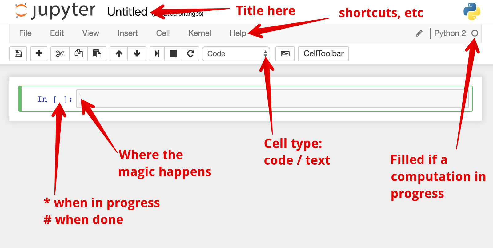
- To execute a cell is Shift + Enter
- To restart the kernel (clean your slate) is Esc + 00
Throughout this tutorial, we will show a few tips for working with the notebook.
Python
Python is a high-level interpreted computing language. Here we outline a few of the basics and common trip-ups. For more information and tutorials, check out the Python Documentation. Note that at the moment, we are using Python 2.7, so those are the docs to follow. In particular, up to chapter 5 at this stage of the tutorials.
Types
Python makes a distinction on types: int, float, and complex:
>>> type(1) == int
True
>>> type(1.) == float
True
>>> type(1j) == complex
True
This is particularly important when doing division:
>>> 1/2
0
Note
If that scares you, you can always use division from the future! from __future__ import division see PEP0238
is integer division, while:
>>> 1./2.
0.5
is floating point division. This is only the case in Python 2, in Python 3, division will return a floating point number.
Counting and Lists
Python uses zero-based indexing:
>>> mylist = [6, 5, 4, 3]
>>> len(mylist)
4
>>> mylist[0]
6
There are a few handy indexing tricks:
>>> mylist[:2] # counting up
[6, 5]
>>> mylist[2:] # starting from
[4, 3]
>>> mylist[-1] # going backwards
3
Loops and List Comprehension
A for loop to append 10 values to a list looks like:
>>> n = 10
>>> a = []
>>> for i in range(n):
... a.append(i)
[0, 1, 2, 3, 4, 5, 6, 7, 8, 9]
or using list comprehension
>>> n = 10
>>> b = [i for i in range(n)]
[0, 1, 2, 3, 4, 5, 6, 7, 8, 9]
Try running these in the notebook and compare the times. To get a better
picture, increase n.
Note
In the notebook, we use the cell magic %%time to track the amount of
time it takes to execute cell
A handy tool for looping over lists is enumerate:
>>> mylist = ['Monty', 'Python', 'Flying', 'Circus'] # python was named after the movie!
>>> for i, val in enumerate(mylist):
... print i, val
0 Monty
1 Python
2 Flying
3 Circus
This is a flavor of some of the flow control for lists in Python, for more details, check out chapters 4, 5 in the Python Tutorial.
If, elif, else
Conditionals in Python are implemented using if, elif, else
>>> # Pick a random number between 0 and 100
>>> import numpy as np
>>> number = (100.*np.random.rand(1)).round() # make it an integer
>>> if number > 42:
...     print '%i is too high'%number
... elif number < 42:
...     print '%i is too low'%number
... else:
...     print 'you found the secret to life. %i'%number
Note that the indentation level matters in python. Logical operators,
or, and are also handy for constructing conditionals
Functions
NumPy

NumPy contains the n-dimensional array machinery for storing and working with
matrices and vectors. To use NumPy, it must first be imported. It is standard
practice to import is as shorthand np.
>>> import numpy as np
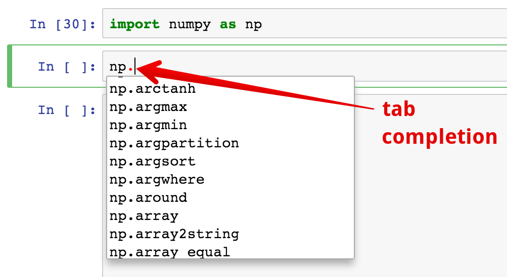
Note
You can use tab completion to look at the attributes of an object
How many dimensions?
NumPy makes a distinction between scalars, vectors and arrays
>>> a = np.array(1) # scalar
>>> print a.shape # has no dimensions
()
>>> b = np.array([1]) # vector
>>> print b.shape # has one dimension
(1,)
>>> c = np.array([[1]]) # array
>>> print c.shape # has two (or more) dimensions
(1, 1)
The shape gives the length of each array dimension. (size
gives you the number of elements)
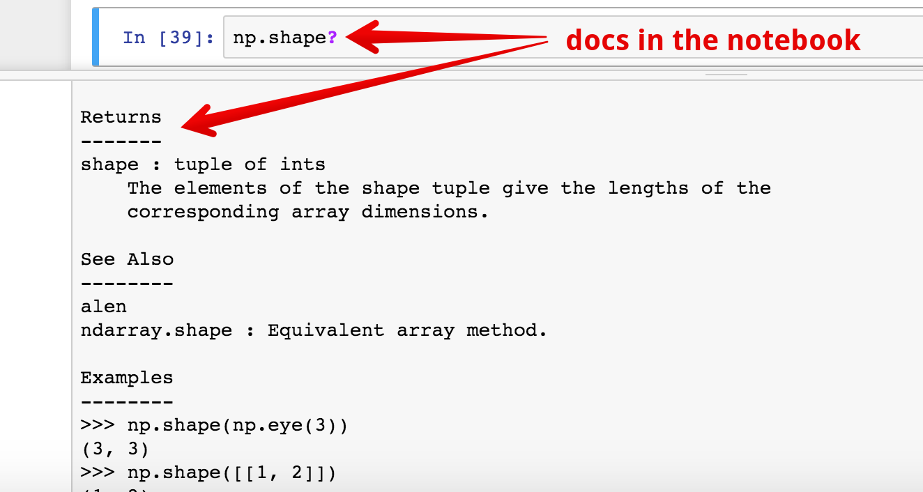
Note
In the notebook, you can query documentation using a ?
This distinction is particularly important when performing linear algebra operations. For instance, if we create a vector:
>>> v = np.random.rand(10)
>>> v.shape
(10,)
and then want to take an inner product, which we expect to output a scalar, one way you might think to do this (spoiler alert: it’s wrong!):
>>> a = v.T * v
>>> a.shape
(10,)
turns out, the concept of a transpose doesn’t matter for vectors, they only have one dimension, so there is no way to exchange dimensions. What we just did was a Hadamard product (element-wise multiplication), so
>>> v.T * v == v * v
True
So how do we take an inner product? (dot)
>>> b = v.dot(v)
>>> b.shape
()
Success! b is a scalar.
What happens if we work with arrays instead?
>>> w = np.random.rand(10,1)
>>> w.shape
(10,1)

Matplotlib
Object Oriented Programming in Python
Also need functions
Class, Inheritance, Properties, Wrappers, and Self