Potential Fields (Magnetics)
Purpose
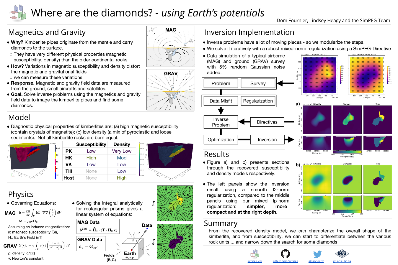
In this tutorial, we demonstrate how to invert magnetic field data in 3D using SimPEG.PF. It simulates a geophysical experiment over a synthetic kimberlite pipe model. The chosen geological model intends to replicate the Tli Kwi Cho kimberlite deposit, NWT. Using SimPEG Directives, we implement a sparse regularization function and recover both a smooth and a compact susceptibility model, which can used to infer geological information at depth. The same example was presented as a poster at Scipy 2016. There is also a notebook available for download here.
Setup
We begin this story with some physics background. We need to establish the connection between rocks magnetic properties and the associated geophysical experiment. Maxwell’s equations for a static electric field and in the absence of free-currents can be written as:
\(\nabla \cdot \mathbf{B} = 0 \\ \nabla \times \mathbf{H} = 0\)
where \(\mathbf{B}\) and \(\mathbf{H}\) correspond to the magnetic flux density and magnetic field respectively. Both quantities are related by:
\(\mathbf{B} = \mu \mathbf{H} \\ \mu = \mu_0 ( 1 + \kappa )\;,\)
where \(\mu\) is the magnetic permeability. In free-space, both \(\mathbf{B}\) and \(\mathbf{H}\) are linearly related by the magnetic permealitity of free-space \(\mu_0\). In matter however, the magnetic flux can be increased proportionally on how easily magnetic material gets polarized, quantified by the magnetic susceptibility \(\kappa\). In a macroscopic point of view, the magnetic property of matter are generally described in terms of magnetization per unit volume such that:
\(\mathbf{M} = \kappa \mathbf{H_s + H_0} + \mathbf{M_r}\;,\)
where \(\mathbf{M}\) can be oriented in any specific direction due to secondary local fields (\(\mathbf{H_s}\)) and/or due to permanent dipole moments (\(\mathbf{M_r}\)). For simplicity we will here assume a purely induced response due to the Earth’s \(\mathbf{H_0}\). Using a few vector identities, we can re-write the magnetic field due to magnetized material in terms of a scalar potential:
\(\phi = \frac{1}{4\pi} \int_{V} \nabla \left(\frac{1}{r}\right) \cdot \mathbf{H}_0 \kappa \; dV\;,\)
where \(r\) defines the relative position between an observer and the magnetic source. Taking the divergence of this potential yields:
\(\mathbf{b} = \frac{\mu_0}{4\pi} \int_{V} \nabla \nabla \left(\frac{1}{r}\right) \cdot \mathbf{H}_0 \kappa \; dV\;.\)
Great, we have a general expression relating any secondary magnetic flux due to magnetic material
Forward Problem
Assuming a purely induced response, we can solve the integral analytically. As derived by Sharma (1966), the integral can be evaluated for rectangular prisms such that:
\(\mathbf{b} = \mathbf{T} \cdot \mathbf{H}_0 \; \kappa\;.\)
Where the tensor matrix \(\bf{T}\) relates the vector magnetization \(\mathbf{M}\) inside a single cell to the components of the field \(\mathbf{b}\) observed at a given location:
\(\mathbf{T} = \begin{pmatrix} T_{xx} & T_{xy} & T_{xz} \\ T_{yx} & T_{yy} & T_{yz} \\ T_{zx} & T_{zy} & T_{zz} \end{pmatrix}\;.\)
In general, we discretize the earth into a collection of cells, each contributing to the magnetic data such that giving rise to a large and dense linear system of the form:
\(\mathbf{b} = \sum_{j=1}^{nc} \mathbf{T}_j \cdot \mathbf{H}_0 \; \kappa_j\;.\)
In most geophysical surveys, we are not collecting all three components, but rather the magnitude of the field, or Total Magnetic Intensity (TMI) data. Because the inducing field is really large, we will assume that the anomalous fields are parallel to \(H_0\):
\(d^{TMI} = \mathbf{\hat H}_0 \cdot \mathbf{b}\;.\)
We then end up with a much smaller system:
\(d^{TMI} = \mathbf{F}\; \boldsymbol{\kappa}\;,\)
where \(\mathbf{F} \in \mathbb{R}^{nd \times nc}\) is our forward operator and \(\kappa\) is the physical property describing the Earth.
Getting started
In order to define a geophysical experiment we need set several important parameters, such as a mesh, data location, inversion parameters and so on. While we could set all of those parameters manually, SimPEG.PF gives the option to work with an input file, capturing all the necessary information to run the inversion. In preparation for this synthetic example, we put together all necessary files and added them to a working directory. The input file can then be loaded and easily accessed through the Driver class:
>> import SimPEG
>> import SimPEG.PF as PF
>> from SimPEG.Utils.io_utils import remoteDownload
>>
>> # Start by downloading files from the remote repository
>> url = 'https://storage.googleapis.com/simpeg/tkc_synthetic/potential_fields/'
>> cloudfiles = ['MagData.obs', 'Mesh.msh',
>>               'Initm.sus', 'SimPEG_PF_Input.inp']
>> driver = PF.MagneticsDriver.MagneticsDriver_Inv(input_file)
>>
>> # Objects loaded from the input file are then accessible like this
>> mesh = driver.mesh
>> initm = driver.m0
Download files from URL...
Retrieving: MagData.obs
Retrieving: Mesh.msh
Retrieving: Initm.sus
Retrieving: SimPEG_PF_Input.inp
Download completed!
The input file looks like this:
| Line | Input | Description |
|---|---|---|
| 1 | Mesh.msh | Mesh file* |
| 2 | Data.obs | Data file* |
| 3 | VALUE -100 | Topography file* | null (all included) |
| 4 | FILE Initm.mod | Starting model* | VALUE ## |
| 5 | VALUE 0 | Reference model* | VALUE ## |
| 6 | DEFAULT | Magnetization file* | DEFAULT |
| 7 | DEFAULT | Cell weight file* | DEFAULT |
| 8 | DEFAULT | Target Chi factor VALUE | DEFAULT (1) |
| 9 | DEFAULT | Scaling parameters for regularization (\(\alpha_s,\alpha_x,\alpha_y,\alpha_z\)) |
| 10 | VALUE 0 1 | Lower and upper bound values |
| 11 | VALUE 0 1 1 1 | Lp-norms applied on model and model gradients (\(p,q_x,q_y,q_z\)) |
| 12 | DEFAULT | Treshold parameter for the norms (\(\epsilon_p,\epsilon_q\)) | DEFAULT |
| Note |
|
We will use each elements later, but for now, this how the inversion is initiated.
Model and Mapping
Since we have already loaded the model in a rectangular mesh, we can plot it with SimPEG’s built-in functions.
Notice that some of the cells in the model are air and show as white. The code will detected the air cells from the VALUE specified on line 3 of the input file. These cells are ignored by the code. Alternatively, the user can input a topography file or an active model specifying the status of each cells (0:inactive, 1:active-dynamic, -1:active-static).
Data
Great, now that we have a mesh and a model, we only need to specify a survey (i.e. where is the data). Once again, an observation file is provided, as specified on Line 2 of the input file. We can now forward model some magnetic data above the synthetic kimberlite.
Error
Unable to execute python code at PF_MAG.rst:228:
no display name and no $DISPLAY environment variable
Inverse Problem
We have generated synthetic data, we now what to see if we can solve the inverse problem. Using the usual formulation, we seek a model that can reproduce the data, let’s say a least-squares measure of the form:
\(\phi_d =\|\mathbf{W}_d \left( \mathbf{F}\;\mathbf{m} - \mathbf{d}^{obs} \right)\|_2^2\;,\)
where \(\mathbf{W}_d\) are estimated data uncertainties The inverse problem is hard because we don’t have great data coverage, and the Earth is big, and there is usually noise in the data. So we need to add something to regularize it. The simplest way to do it is to penalize solutions that won’t make sense geologically, for example to assume that the model is small and smooth. Most inversion codes use the l2-norm measure such that:
\(\phi_m = {\| \mathbf{W}_s \;( \mathbf{m - m^{ref}})\|}^2_2 + \sum_{i = x,y,z} {\| \mathbf{W}_i \; \mathbf{G}_i \; \mathbf{m}\|}^2_2\)
where \(m^{ref}\) is any a priori knowledge that we might have about the solution and \(\mathbf{G}_x, \mathbf{G}_y, \mathbf{G}_z\) are finite difference operators measuring the model spatial gradients along orthogonal directions. In a purely unconstrained case, \(m^{ref}\) is usually equal to some background value (i.e. zero susceptibility). The full objective function to be minimized can be written as:
\(\phi (m) = \phi_d + \beta \phi_m\)
which will yield our usual function that minimize the data error and model structure. The trade-off parameter \(\beta\) is adjusted in order to get a good balance between data misfit and model
We propose a fancier regularization function that can allow to recover sparse and blocky solutions. Starting with the well known Ekblom norm:
\(\phi_m = \sum_{i=1}^{nc} {(x_i^2 + \epsilon^2)}^{p/2}\)
where \(x_i\) denotes some function of the model parameter, and \(\epsilon\) is a small value to avoid singularity as \(m\rightarrow0\).
For p=2, we get the usual least-squares measure and we recover the regularization presented above. For \(p \leq 1\), the function becomes non-linear which requires some tweaking. We can linearize the function by updating the penality function iteratively, commonly known as an Iterative Re- weighted Least-Squares (IRLS) method. The regularization function becomes:
\(\phi_m^{(k)} = \frac{1}{2}\sum_{i=1}^{nc} r_i \; x_i^2\)
where we added the superscript \(\square^{(k)}\) to denote the IRLS iterations. The weights \(r(x)\) are computed from model values obtained at a previous iteration such that:
\({r}_i ={\Big( {({x_i}^{(k-1)})}^{2} + \epsilon^2 \Big)}^{p/2 - 1}\)
where \({r}(x) \in \mathbb{R}^{nc}\).
In matrix form, our objective function simply becomes:
\(\phi(m) = \|\mathbf{W}_d \left( \mathbf{F}\;\mathbf{m} - \mathbf{d}^{obs} \right)\|_2^2 + \beta \Big [ {\| \mathbf{W}_s \;\mathbf{R}_s\;( \mathbf{m - m^{ref}})\|}^2_2 + \sum_{i = x,y,z} {\| \mathbf{W}_i\; \mathbf{R}_i \; \mathbf{G}_i \; \mathbf{m}\|}^2_2 \Big ]\)
where the IRLS weights \(\mathbf{R}_s\) and \(\mathbf{R}_i\) are diagonal matrices defined as:
\({R}_{s_{jj}} = \sqrt{\eta_p}{\Big[ {({m_j}^{(k-1)})}^{2} + \epsilon_p^2 \Big]}^{(p/2 - 1)/2}\)
\({R}_{i_{jj}} = \sqrt{\eta_q}{\Big[ {\left ({{(G_i\;m^{(k-1)})}_j }\right)}^{2} + \epsilon_q^2 \Big]}^{(q/2 - 1)/2}\)
\(\eta_p = {\epsilon_p}^{(1-p/2)}\;,\) \(\eta_q = {\epsilon_q}^{(1-q/2)}\)
we added two scaling parameters \(\eta_p\) and \(\eta_q\) for reasons that we won’t dicuss here, but turn out to be important to get stable solves.
In order to initialize the IRLS and get an estimate for the stabilizing parameters \(\epsilon_p\) and \(\epsilon_q\), we first invert with the smooth \(l_2\)-norm. Once the target data misfit has been achieved, the inversion switches to the sparse regularization. This way we get a good starting point, hopefully close enough to the true solution. The whole IRLS process is implemented with a directive added to the inversion workflow.
Error
Unable to execute python code at PF_MAG.rst:380:
Now we can plot sections and compare the smooth and compact models with the true solution.
Summary
We have inverted magnetic field data over a synthetic kimberlite pipe, using both a smooth and compact penalty. The smooth model gives a conservative and robust estimate of the kimberlite pipe location, as well as providing an excellent starting point for the sparse regularization. The compact model on the other hand gives a much closer estimate of susceptibility values and shape of the magnetic anomaly. More details about the scaled IRLS method can be found in this thesis.