DC resistivity
Purpose
Understand basic setup and physics of a direct current (DC) resistivity survey within the context of a kimberlite exploration. Run DC forward modelling and inversion using SimPEG-Static package.

Set-up
The physical behavior of DC resistivity survey is governed by the steady-state Maxwell’s equations:
where: - \(\vec{j}\): Current density (A/m \(^2\))
- \(\vec{e}\): Electric field (V/m)
- \(I_0\): Current (A)
- \(\delta\): Volumetric delta function (m \(^{-3}\))
Consider a simple gradient array having a pair of A (+) and B (+) current electrodes (Tx) with multiple M (+) and N (-) potential electrodes (Rx). Using giant battery (?), we setup a significant potential difference allowing electrical currents to flow between the A to B electrodes. If the earth includes conductors or resistors, these will distorts current flow, and measured potential differences on the surface electrodes (MN) will be reflective of those distortions. Typically kimberlitic pipes (including those containing diamonds!) will be more conductive than the background rock (granitic), hence, the measured potential difference will be low. That is, contrasts in electrical conductivity between different rocks induce anomalous voltages. From the observed voltages, we want to estimate conductivity distribution of the earth. We use a geophysical inversion technique to do this procedure.
We work through each step of geophysical inversion using SimPEG-Static package under SimPEG’s framework having two main items: a) Forward simulation and b) Inversion.
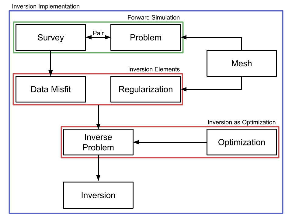
Fig. 1 SimPEG’s framework
Forward simulation
A forward simulation of a DC experiment requires Survey and Problem classes. We need to the pass current and potential electrode locations to a DC survey class. The physical behavior of DC fields and fluxes are governed by the static Maxwell’s equations. To numerically work with these equations, we use the DC problem class, which handles this by solving a corresponding partial different equation in a discrete space. For this, the earth needs to be discretized to solve corresponding partial differential equation. The Problem class computes fields in full discretized domain, and the Survey class evaluates data at potential electrodes using the fields. The Survey and Problem classes need to share information hence, we pair them.
Mesh
We use a 3D tensor mesh to discretize the earth having 25x25x25 m core cell size. Smaller vertical size of the cell (dz) is used close to the topographic surface (12.5 m), and padding cells are used to satisfies the natural boundary condition imposed.
Survey
We use a simple gradient array having a pair of current electrodes (AB), and multiple potential electrodes (MN). The lengths of AB and MN electrodes are 1200 and 25 m, respectively.

Fig. 2 Gradient array
Once we have obtained locations of AB (Src) and MN (Rx) electrodes, we can generate Survey class:
from SimPEG.EM.Static import DC

# Create Src and Rx classes for DC problem
Aloc1_x = np.r_[-600., 0, 0.] + np.r_[xc, yc, zc]
Bloc1_x = np.r_[600., 0, 0.] + np.r_[xc, yc, zc]

# Rx locations (M-N electrodes, x-direction)
x = mesh.vectorCCx[np.logical_and(mesh.vectorCCx>-300.+ xc, mesh.vectorCCx<300.+ xc)]
y = mesh.vectorCCy[np.logical_and(mesh.vectorCCy>-300.+ yc, mesh.vectorCCy<300.+ yc)]
# Grid selected cell centres to get M and N Rx electrode locations
Mx = Utils.ndgrid(x[:-1], y, np.r_[-12.5/2.])
Nx = Utils.ndgrid(x[1:], y, np.r_[-12.5/2.])

rx = DC.Rx.Dipole(Mx, Nx)
src = DC.Src.Dipole([rx], Aloc1_x, Bloc1_x)

# Form survey object using Srcs and Rxs that we have generated
survey = DC.Survey([src])
Fields and Data
By solving the DC equations, we compute electrical potential (\(\phi\)) at every cell. The Problem class does this, but it still requires survey information hence we pair it to the Survey class:
# Define problem and set solver
problem = DC.Problem3D_CC(mesh)

problem.Solver = MumpsSolver
# Pair problem and survey
problem.pair(survey)
Here, we used DC.Problem3D_CC, which means 3D space and \(\phi\) is
defined at the cell center. Now, we are ready to run DC forward modelling! For
this modelling, inside of the code, there are two steps:
- Compute fields (\(\phi\) at every cells)
- Evaluate at Rx location (potential difference at MN electrodes)
Consider two conductivity models:
- Homogeneous background below topographic surface:
sigma0(\(10^{-4}\) S/m) - Includes diamond pipes:
sigma(S/m)
# Read pre-generated conductivity model in UBC format
sigma = mesh.readModelUBC("VTKout_DC.dat")
# Identify air cells in the model
airind = sigma == 1e-8
# Generate background model (constant conductiivty below topography)
sigma0 = np.ones_like(sigma)*1e-4
sigma0[airind] = 1e-8
Then we compute fields for both conductivity models:
# Forward model fields due to the reference model and true model
f0 = problem.fields(sigma0)
f = problem.fields(sigma)
Now f and f0 are Field objects including computed \(\phi\)
everywhere. However, this Field object know how to compute both
\(\vec{e}\), \(\vec{j}\), and electrical charge, \(\int_V \rho_v
dV\) (\(\rho_v\) is volumetric charge density). Note that if we know
\(\phi\), all of them can be computed for a corresponding source:
phi = f[src, 'phi']
e = f[src, 'e']
j = f[src, 'j']
charge = f[src, 'charge']
Since the field object for the background model is generic, we can obtain secondary potential:
# Secondary potential
phi0 = f0[src, 'phi']
phi_sec = phi - phi0
We present plan and section views of currents, charges, and secondary potentials in Fig. 3.

Fig. 3 DC fields. Left, middle, and right panels show currents, charges, and secondary potentials.
Current flows from A (+) to B (-) electrode (left to right). Kimberlite pipe should be more conductive than the background considering more currents are flowing through the pipe (See distortions of the current path in the left panel).
The distribution of electrical charges (the middle panel) supports that the pipe is conductive since left and right side of the pipe has negative and positive charges, respectively. In addition, charges only built on the boundary of the conductive pipe.
The secondary potential (the right panel) is important since it shows response from the kimberlite pipe, which often called “Anomalous potential”. Usually, removing background response is a good way to see how much anomalous response could be obtained for the target.
On the other hand, we cannot measure those fields everywhere but measure potential differences at MN electrodes (Rx) hence we need to evaluate them from the fields:
# Get observed data
dobs = survey.dpred(sigma, f=f)
If the field has not been computed then we do:
# Get observed data
dobs = survey.dpred(sigma)
This will compute the field inside of the code then evaluate for data at Rx locations. Below image shows the computed DC data. Smaller potentials are obtained at the center locations, which implies the existence of conductive materials. Current easily flows with conductive materials, which means less potential is required to path through them, hence for resistive materials we get greater potential difference measured on the surface. The measured potential provides some idea of the earth; however, this is not enough, we want a 3D distribution of the conductivity!

Fig. 4 DC data.
Inversion Elements
Our goal here is finding a 3D conductivity model which explains the observed data shown in Fig. 4. Inversion elements (red box in Fig. 1) will handle this task with an ability to simulate forward problem. We go through each element and briefly explain.
Mapping
For the simulation, we used a 3D conductivity model, with a value defined in every cell center location. However, for the inversion, we may not want to estimate conductivity at every cell. For instance, our domain include some air cells, and we already know well about the conductivity of the air (\(10^{-8} \approx 0\)) hence, those air cell should be excluded from the inversion model, \(m\). Accordingly, a mapping is required moving from the inversion model to conductivity model defined at whole discrete domain:
In addition, conductivity is strictly positive and varies logarithmically, so we often use log conductivity as our inversion model (\(m = log (\sigma)\)). Our inversion model is log conductivity only defined below the subsurface cells, and this can be expressed as
where \(\mathcal{M}_{act}(\cdot)\) is a InjectActiveCells map, which
takes subsurface cell and surject to full domain including air cells, and
\(\mathcal{M}_{exp}(\cdot)\) is an ExpMap map takes log conductivity
to conductivity. Combination of two maps are required to get \(\sigma\)
from \(m\), which can be codified as
# from log conductivity to conductivity
expmap = Maps.ExpMap(mesh)
# from subsurface cells to full 3D cells
actmap = Maps.InjectActiveCells(mesh, ~airind, np.log(1e-8))
mapping = expmap*actmap
Generated mapping should be passed to Problem class:
# Generate problem with mapping
problem = DC.Problem3D_CC(mesh, sigmaMap=mapping)
Data Misfit
Finding a model explaining the observed data requires a measure between observed (\(\mathbf{d}^{obs}\)) and predicted data (\(\mathbf{d}^{dpred}\)):
where \(\mathbf{W}_d = \mathbf{diag}( \frac{1}{\% | \mathbf{d}^{obs} |+\epsilon} )\) is the data weighting matrix. Uncertainty in the observed data is approximated as \(\% | \mathbf{d}^{obs} |+\epsilon\).
# percentage and floor for uncertainty in the observed data
std, eps = 0.05, 1e-3
survey.std = std
survey.eps = eps
survey.dobs = dobs

# Define datamisfit portion of objective function
dmisfit = DataMisfit.l2_DataMisfit(survey)
Regularization
The objective function includes both data misfit and regularization terms, \(\phi_m\) :
We use Tikhonov-style regularization including both smoothness and smallness terms. For further details of this See XXX.
In addition, considering the geometry of the gradient array: a single source and distributed receivers, this specific DC survey may not have much depth resolution similar to magnetic and gravity data. Depth weighting (\(\frac{1}{(z-z_0)^3}\)) is often used to handle this. And with this weight we form Regularization class:
# Depth weighting
depth = 1./(abs(mesh.gridCC[:,2]-zc))**1.5
depth = depth/depth.max()

# Define regulatization (model objective function)
reg = Regularization.Simple(mesh, mapping=regmap, indActive=~airind)
reg.wght = depth[~airind]
reg.alpha_s = 1e-1
reg.alpha_x = 1.
reg.alpha_y = 1.
reg.alpha_z = 1.
Optimization
To minimize the objective function, an optimization scheme is required. The Optimization class handles this, and we use Inexact Gauss Newton Scheme CITExxx.
opt = Optimization.InexactGaussNewton(maxIter = 20)
InvProblem
Both DatamMisfit and Regularization classes are created, and an Optimization is chosen. To pose the inverse problem, they need to be declared as an optimization problem:
The InvProblem class can be set with DatamMisfit, Regularization and Optimiztion classes.
invProb = InvProblem.BaseInvProblem(dmisfit, reg, opt)
Inversion
We have stated our inverse problem, but a conductor is required, who directs our inverse problem. Directives conducts our Inversion. For instance, the trade-off parameter, \(\beta\) needs to be estimated, and sometimes cooled in the inversion iterations. A target misfit is need to be set usually upon discrepancy principle (\(\phi_d^\ast = 0.5 N_d\), where \(N_d\) is the number of data).
# Define Directives
betaest = Directives.BetaEstimate_ByEig(beta0_ratio=1e0)
beta = Directives.BetaSchedule(coolingFactor=5, coolingRate=2)
target = Directives.TargetMisfit()

# Define Inversion class
inv = Inversion.BaseInversion(invProb, directiveList=[beta, betaest, target])
Run
Now we all set. The initial model is assumed to be homogeneous.
# Create inital and reference model (1e-4 S/m)
m0 = np.ones(mesh.nC)[~airind]*np.log(1e-4)

# Run inversion
mopt = inv.run(m0)
The inversion runs and reaches to the target misfit, hence we fit the observed data.

Fig. 5 Observed and Predicted DC data.
A 3D conductivity model is recovered and compared with the true conductivity model. A conductive pipe at depth is recovered!

Fig. 6 True and recovered conductivity models.